Table of Contents
- 1. Introduction
- 2. Hibari’s Main Features in Broad Detail
- 2.1. Distributed system
- 2.2. Scalable system
- 2.3. Durable updates
- 2.4. Consistent updates
- 2.5. Lockless client API
- 2.6. High availability
- 2.7. Multiple Client Protocols
- 2.8. High performance
- 2.9. Automatic repair
- 2.10. Dynamic configuration
- 2.11. Data rebalancing
- 2.12. Heterogeneous hardware support
- 2.13. Micro-Transactions
- 2.14. Per-table configurable performance options
- 3. Getting Started with Hibari (INCOMPLETE)
- 4. Building A Hibari Database
- 5. Hibari Architecture
- 6. The Admin Server Application
- 7. Hibari System Information: Configuration Files, Etc.
- 8. The Life of a (Logical) Brick
- 9. Dynamic Cluster Reconfiguration
- 10. The Partition Detector Application
- 11. Backup and Disaster Recovery
- 12. Hibari Application Logging
- 13. Hardware and Software Considerations
- 14. Administering Hibari Through the API
- 14.1. Add a New Table: brick_admin:add_table()
- 14.2. Delete a Table
- 14.3. Change a Chain: Add or Remove Bricks
- 14.4. Change a Table: Add/Remove Chains
- 14.5. Change a Table: Change Chain Weighting
- 14.6. Admin Server API
- 14.7. Scoreboard API
- 14.8. Chain Monitor API
- 14.9. Changing Chain Length: Examples
- 14.10. Creating and Rebalancing Chains: Examples
This document is under re-construction - beware! |
There exists a dichotomy in modern storage products. Commodity storage is inexpensive, but unreliable. Enterprise storage is expensive, but reliable. Large capacities are present in both enterprise and commodity class. The problem, then, becomes how to leverage inexpensive commodity hardware to achieve high capacity enterprise class reliability at a fraction of the cost.
This problem space has been researched extensively, especially in the last few years: in academia, the commercial sector, and by open source community. Hibari uses techniques and algorithms from this research to create a solution which is reliable, cost effective, and scalable.
Hibari is key-value store. If a key-value store were represented as an SQL table, it would be defined as:
SQL-like definition of a generic key value store.
CREATE TABLE foo (
    BLOB key;
    BLOB value;
) PRIMARY KEY key;
In truth, each key stored in Hibari has three additional fields associated with it. See Section 4.2, “The Hibari Data Model” and Hibari Contributor’s Guide for details.
Hibari was originally written by Cloudian, Inc. (formerly Gemini Mobile Technologies) to support mobile messaging and email services. Hibari was released outside of Cloudian under the Apache Public License version 2.0 in July 2010.
Hibari has been deployed by multiple telecom carriers in Asia and Europe. Hibari may lack some features such as monitoring, event and alarm management, and other "production environment" support services. Since telecom operator has its own data center support infrastructure, Hibari’s development has not included many services that would be redundant in a carrier environment. We hope that Hibari’s release to the open source community will close those functional gaps as Hibari spreads outside of carrier data centers.
Cloudian, Inc. provides full support, consulting, and development services for Hibari. Please see the Hibari NOSQL at Cloudian web site for more information.
- A Hibari cluster is a distributed system.
- A Hibari cluster is linearly scalable.
- A Hibari cluster is highly available.
- All updates are durable.
- All updates are strongly consistent.
- All client operations are lockless.
- A Hibari cluster’s performance is excellent.
- Multiple client access protocols are available.
- Data is repaired automatically after a server failure.
- Cluster configuration can be changed at any time.
- Data is automatically rebalanced.
- Heterogeneous hardware support is easy.
- Micro-transactions simplify creation of robust client applications.
- Per-table configurable performance options are available.
We strongly believe that "ACID" and "BASE" properties exist on a spectrum and are not exclusively one or the other (black-or-white) properties. |
Most database users and administrators are familiar with the acronym ACID: Atomic, Consistent, Independent, and Durable. Now, consider an alternative method of storing and managing data, BASE:
- Basically available
- Soft state
- Eventually consistent
For an exploration of ACID and BASE properties (at ACM Queue), see:
BASE: An Acid Alternative
Dan Pritchett
ACM Queue, volume 6, number 3 (May/June 2008)
ISSN: 1542-7730
http://queue.acm.org/detail.cfm?id=1394128
When both strict ACID and strict BASE properties are placed on a spectrum, they are at the opposite ends. However, a distributed database system can fit anywhere in the middle of the spectrum.
A Hibari cluster lies near the ACID end of the ACID/BASE spectrum. In general, Hibari’s design will always favors consistency and durability of updates at the expense of 100% availability in all situations.
Eric Brewer’s "CAP Theorem", and its proof by Gilbert and Lynch, is a tricky thing. It’s nearly impossible to cleanly apply the purity of logic to the dirty world of real, industrial computing systems. We strongly suggest that the reader consider the CAP properties as a spectrum, one of balances and trade-offs. The distributed database world is not black and white, and it is important to know where the gray areas are. |
See the Wikipedia article about the CAP theorem for a summary of the theorem, its proof, and related links.
CAP Theorem (postulated by Eric Brewer, Inktomi, 2000)
Wikipedia
http://en.wikipedia.org/wiki/CAP_theorem
Hibari chooses the C and P of CAP. It utilizes chain replication technique and it always guarantees strong consistency. Hibari also includes an Erlang/OTP application specifically for detecting network partitions, so that when a network partition occurs, the brick nodes in the opposite side of the partition with the active master will be removed from the chains to keep the strong consistency guarantee.
See Section 6.4, “Admin Server and Network Partition” for details.
Copyright © 2005-2013 Hibari developers. All rights reserved.
Licensed under the Apache License, Version 2.0 (the "License");
you may not use this file except in compliance with the License.
You may obtain a copy of the License at

    http://www.apache.org/licenses/LICENSE-2.0

Unless required by applicable law or agreed to in writing, software
distributed under the License is distributed on an "AS IS" BASIS,
WITHOUT WARRANTIES OR CONDITIONS OF ANY KIND, either express or implied.
See the License for the specific language governing permissions and
limitations under the License.Multiple machines can participate in a single cluster. The maximum size of a Hibari cluster has not yet been determined. A practical limit of approximately 200-250 nodes is likely.
Any server node can handle any client request, forwarding a request to the correct server node when necessary. Clients maintain enough state to send their queries directly to the correct server node in all common cases.
The total storage and processing capacity of a Hibari cluster increases linearly as machines are added to the cluster.
Every key update is written and flushed to stable storage (via the
fsync() system call) before sending acknowledgments to the client.
After a key’s update is acknowledged, no client in the cluster can see an older version of that key. Hibari uses the "chain replication" algorithm to maintain consistency across all replicas of a key.
All data written to disk include MD5 checksums; the checksums are validated on each read to avoid sending corrupted data to the client.
The Hibari client API requires that all operations (read queries operations and/or update operations) be self-contained within a single client request. Therefore, locks are not implemented because they are not required.
Inside Hibari, each key-value pair also contains a “timestamp” value. A timestamp is an integer. Each time the key is updated, the timestamp value must increase. (This requirement is enforced by all server nodes.)
In many database systems, if a client requires guarantees that a key has not changed since the last time it was read, then the client acquires a lock (or lease) on the key. In Hibari, the client’s update specifies the timestamp of the last read attempt of the key:
- If the timestamp matches the server, the operation is permitted.
- If the timestamp does not match the server’s timestamp, then the operation is not permitted, and the new timestamp is returned to the client.
It is recommended that all Hibari nodes use NTP to synchronize their system clocks. The simplest Hibari client API uses timestamps based upon the OS system clock for timestamp values. This feature can be bypassed, however, by using a slightly more complex client API.
However, Hibari’s overload detection and work-dumping algorithms will use the OS system clock, regardless of which client API is used. All system clocks, client and server, be synchronized to be within roughly 1 second of each other.
Each key can be replicated multiple times (configurable on a per-table basis). As long as one copy of the key survives, all operations on that key are permitted. A cluster can survive multiple cluster node failures and still maintain full data integrity.
The cluster membership application, called the Hibari Admin Server, runs as an active/standby application on one or more of the server nodes. The Admin Server’s configuration and private state are also maintained in Hibari server nodes. Shared storage such as NFS, shared SCSI/Fibre Channel LUNs, or replicated block devices are not required.
If the Admin Server fails and is restarted on a standby node, the rest of the cluster can continue normal operation. If another brick fails while the Admin Server is restarting, then clients may see service interruptions (usually in the form of timeouts) until the Admin Server has finished restarting and can react to the failure.
Hibari supports many client protocols for queries and updates:
- A native Erlang API, via Erlang’s native message-passing mechanism
- Amazon S3 protocol, via HTTP
- UBF, Joe Armstrong’s “Universal Binary Format” protocol, via TCP
- UBF via several minor variations of TCP transport
- UBF over JSON-RPC, via HTTP
- JSON-encoded UBF, via TCP
Protocols under development:
- Memcached, via TCP
- UBF over Thrift, via TCP
- UBF over Protocol Buffers, via TCP
Most of the client access protocols are implemented using the
Erlang/OTP application behavior. By separating each access protocol
into separate OTP applications, Hibari’s packaging is quite flexible:
packaging can add or remove protocol support as desired. Similarly,
protocols can be stopped and started at runtime.
Hibari’s performance is competitive with other distributed, non-relational databases such as HBase and Cassandra, when used with similar replication and durability configurations. Despite the constraints of durable writes and strong consistency, Hibari’s performance can exceed those databases on some workloads.
The metadata of all keys stored by the brick, called the “key catalog”, are stored in RAM to accelerate commonly-used operations. In addition, non-zero values of the "expiration_time" and non-empty values of "flags" are also stored in RAM (see SQL-like definition of a Hibari table). As a consequence, a multi-million key brick can require many gigabytes of RAM. |
Replicas of keys are automatically repaired whenever a cluster node crashes and restarts.
The number of replicas per key can be changed without service interruption. Likewise, replication chains can be added or removed from the cluster without service interruption. This permits the cluster to grow (or shrink) as workloads change. See Section 9.4, “Chain Migration: Rebalancing Data Across Chains” for more details.
Keys will be automatically be rebalanced across the cluster without service interruption. See Section 9.4, “Chain Migration: Rebalancing Data Across Chains” for more details.
Each replication chain can be assigned a weighting factor that will increase or decrease the percentage of a table’s key space relative to all other chains. This feature can permit use of cluster nodes with different CPU, RAM, and/or disk capacities.
Under limited circumstances, operations on multiple keys can be given transactional commit/abort semantics. Such micro-transactions can considerably simplify the creation of robust applications that keep data consistent despite failures by both clients and servers.
Each Hibari table may be configured with the following options to enhance performance … though each of these options has a corresponding price to pay.
- RAM-based storage: All data (both keys and values) may be stored in RAM, at the expense of increased RAM consumption. Disk is used still used to log all updates, to protect against a catastrophic power failure.
-
Asynchronous writes: Use of the
fsync()system call can be disabled to improve performance, at the expense of data loss in a system crash or power failure. - Non-durable updates: All update logging can be disabled to improve performance, at the expense of data loss when all nodes in a replication chain crash.
draft
Don’t forget to mention the recommendation of 2 physical network interfaces. |
Hibari is a key-value database. Unlike a relational DBMS, Hibari applications do not need to create a schema. The only application requirement is that all its tables be created in advance, see Section 4.5, “Creating New Tables” below.
If a Hibari table were represented within an SQL database, it would look something like this:
SQL-like definition of a Hibari table.
CREATE TABLE foo (
    BLOB key;
    BLOB value;
    INTEGER timestamp;                  -- Monotonically increasing
    INTEGER expiration_time;            -- Usually zero
    LIST OF ATOMS_AND_TWO_TUPLES flags; -- Metadata stored in RAM for speed
) PRIMARY KEY key;
Hibari table names use the Erlang data type “atom”. The types of all key-related attributes are presented below.
Table 1. Types of Hibari table key-value attributes
| Attribute Name | Erlang data type | Storage Location | Description |
|---|---|---|---|
Key | binary | RAM | A binary blob of any size, though due to RAM storage the key should be small enough for all keys to fit in RAM. |
Value | binary | RAM or disk | A binary blob of any size, though practical constraints limit value blobs to 16MB or so. |
Timestamp | integer | RAM | A monotonically increasing counter, usually (but not always) based on the client’s wall-clock time. Updating a key with a timestamp smaller than the key’s current timestamp is not permitted. |
Expiration Time | integer | RAM | A UNIX |
Flags | list | RAM | This attribute cannot be represented in plain SQL. It is a list of atoms and/or {atom(), term()} pairs. Heavy use of this attribute is discouraged due to RAM-based storage. |
"Storage location = RAM" means that, during normal query handling, data is retrieved from a copy in RAM. All modifications of any/all attributes of a key are written to the write-ahead log to prevent data loss in case of a cluster-wide power failure. See Section 5.2, “Write-Ahead Logs” for more details.
"Store location = disk" means that the value of the attribute is not
stored in RAM. Metadata in RAM contains a pointer to the attribute’s
location:file #, byte offset, and length. A log sequence file inside
the common log must be opened, call lseek(2), and then read(2) to
retrieve the attribute.
- Best case
- Zero disk seeks are required to read a key’s value blob from disk, because all data in question is in the OS’s page cache.
- Typical case
- One seek and read is required: the file’s inode info is cached, but the desired file page(s) is not cached.
- Worse case
- The file system will need to perform additional seeks and reads to read intermediate directory data, inode, and indirect storage block data within the inode.
The practical constraints on maximum value blob size are affected by
total blob size and frequency of large blob access. For example,
storing an occasional 64MB value blob is different than a 100% write
workload of 100% 64MB value blobs. The Hibari client API does not
have a method to update or fetch less than the entire value blob, so a
brick can be blocked for many seconds if it tried to operate on (for
example) even a single 4GB blob. In addition, other processes can be
blocked by 'busy_dist_port' events while processing big value blobs.
Hibari’s basic client operations are enumerated below.
-
add - Set a key/value/expiration/flags only if the key does not already exist.
-
delete - Delete a key
-
get - Get a key’s timestamp and value
-
get_many - Get a range of keys
-
replace - Set a key/value/expiration/flags only if the key does exist
-
set - Set a key/value/expiration/flags
-
txn - Start of a micro-transaction
Each operation can be accompanied by operation-specific flags. Some of these flags include:
-
witness -
Do not return the value blob. (
get,get_many) -
must_exist - Abort micro-transaction if key does not exist.
-
must_not_exist - Abort micro-transaction if key does exist.
-
{testset, TS} -
Perform the action only if the key’s current timestamp
exactly matches
TS. (delete,replace,set, micro-transaction)
For details of these operations and lesser-used per-operation flags, see:
Hibari does not support automatic indexing of value blobs. If an application requires indexing, the application must build and maintain those indexes.
New tables can be created by two different methods:
- Via the Admin Server’s status server. Follow the "Add a table" link at the bottom.
- Using the Erlang shell.
For details on the Erlang shell API and detailed explanations of the table options presented in the Admin server’s HTTP interface, see the Hibari Contributor’s Guide
From a logical point of view, Hibari’s architecture has three layers:
- Top layer: consistent hashing
- Middle layer: chain replication
- Bottom layer: the storage brick
This section discusses each of these major layers in detail, starting from the bottom and working upward.


The word "brick" has two different meanings in a Hibari system:
- An entire physical machine that has Hibari software installed, configured, and (hopefully) running.
- A logical software entity that runs inside the Hibari application that is responsible for managing key-value pairs.
The phrase "physical brick" and "machine" are interchangeable, most of the time. Hibari is designed to react correctly to the failure of any part of the machine that the Hibari application is running:
- disk
- power supply
- CPU
- network
Hibari is designed to take advantage of low-cost, off-the-self commodity servers.
A physical brick is the basic unit of failure. Data replication (via the chain replication algorithm) is responsible for protecting data, not redundant equipment such as dual power supplies and RAID disk subsystems. If a physical brick crashes for any reason, copies of data on other physical bricks can still be used.
It is certainly possible to decrease the chances of data loss by using physical bricks with more expensive equipment. Given the same number of copies of a key-value pair, the chances of data loss are less if each brick has multiple power supplies and RAID 1/5/6/10 disk. But risk of data loss can also be reduced by increasing the number of data replicas ("chain length") using cheaper, non-redundant server hardware.
A logical brick is a software entity that runs within a Hibari application instance on a physical brick. A single Hibari physical brick can support dozens or (potentially) hundreds of logical bricks, though limitations of CPU, RAM, and/or disk capacity can impose a smaller limit.
A logical brick maintains RAM and disk data structures to store a collection of key-value pairs. The keys are maintained in lexicographic sorting order.
The replication technique used by Hibari, chain replication, maintains identical copies of key-value pairs across multiple logical bricks. The number of copies of a key-value pair is exactly equal to the length of the chain. See the next subsection below for more details.
It is possible to configure Hibari to place all of the logical bricks for the same chain onto the same physical brick. This practice can be useful in a developer’s environment, but it is impractical for production networks: such a configuration does not have any physical redundancy, and therefore it poses a greater risk of data loss.
By default, all logical bricks will record all updates to a “write-ahead log”. Used by many database systems, a write-ahead log (WAL) appears to be an infinitely-sized log where all important events (e.g. all write and delete operations) are appended to the end of the log. The log is considered “write-ahead” if a log entry is written prior to any significant processing by the application.
Two types of write-ahead logs are used by the Hibari application. These logs cooperate with each other to provide several benefits to the logical brick.
There are two types of write-ahead logs:
-
The shared "common log". This single write-ahead log instance provides
durability guarantees to all logical bricks within the server node
via the
fsync()system call. - Individual “private logs”. Each logical brick maintains its own private write-ahead log instance. All metadata regarding keys in the logical brick are stored in the logical brick’s private log.
All updates are written first to the common log, usually in a synchronous manner. At a later time, update metadata is lazily copied from the common log to the corresponding brick’s private log. Value blobs (for bricks that store value blobs on disk) will remain in the common log and are managed by the “scavenger”, see Section 8.7, “The Scavenger”.
 |
The two log types cooperate to support a number of useful properties.
- Data durability in case of system crash or power failure. All synchronous writes to the “common log” are guaranteed to be flushed to stable storage.
-
Performance enhancement by limiting
fsync()usage. After a logical brick writes data to the common log, it will request anfsync(). The common log will combinefsync()requests from multiple bricks into a single system call. - Performance enhancement at logical brick startup. A brick’s private log stores only that bricks key metadata. Therefore, at startup time, the logical brick does not scan data maintained by other logical bricks. This can be a very substantial time savings as the amount of metadata managed by all logical bricks grows over time.
-
Performance enhancement by separating synchronous writes from
asynchronous writes. If the common log’s storage is on a separate
device, e.g. a write-optimized flash memory block device, then all
of the
fsync()calls can finish much faster. During later processing of the asynchronous/lazy copying of key metadata from the common log to individual private logs can take advantage of OS dirty page write coalescing and other I/O optimizations without interference byfsync(). These copies are performed roughly once per second.
Each write-ahead log is stored on disk as a collection of large files (default = 100MB each). Each file in the log is identified by a “log sequence number” and is called a “log sequence file”.
Log sequence files are append-only and are never written again. Consequently, data in a log sequence file is never overwritten. Any disk space reclaimed by checkpoint and scavenger operations is done by copying data from old log sequence files and appending to new log sequence files. Once the new log sequence file(s) is flushed to stable storage, the old log sequence file(s) can be deleted.
When a log sequence file reaches its maximum size, the current log file is closed and a new one is opened with a monotonically increasing log serial number.
All log files for a write-ahead log are grouped under a single
the brick or of the common log. These directories are stored under
the var/data subdirectory of the application’s installation path,
/usr/local/TODO/TODO/var/data (by default).
The maximum log file size (brick_max_log_size_mb in the
central.conf file) is advisory only and is not enforced as a hard
limit.
In practice, infinite storage is not yet available. The Hibari system uses two mechanisms to reclaim unused disk space:
- The “checkpoint” mechanism, see Section 8.6, “Brick Checkpoint Operations”.
- The “scavenger” mechanism, see Section 8.7, “The Scavenger”.
Each item written in a write-ahead log is assigned a serial number. If the brick is in “standalone” or “head” roles, then the serial number will be assigned by that brick. For downstream bricks, the serial number assigned by the “head” brick will be used.
The serial number mechanism is used to ensure that a single unique ordering of log items will be written to each brick log. In certain failure cases, log items may be re-sent down the chain a second time, see the section called “Failure of a middle brick”.
A chain is the unit of data replication used by the “chain replication” technique as described in this paper:
Chain Replication for Supporting High Throughput and Availability
Robbert van Renesse and Fred B. Schneider
USENIX OSDI 2004 conference proceedings
http://www.usenix.org/events/osdi04/tech/renesse.html
Data replication algorithms can be separated into two basic families:
- State machine replication
- Quorum replication
The chain replication algorithm is from the state machine family of replication algorithms. It is a variation of the familiar “master/slave” replication algorithm, where all updates are sent to a master node and then copies are sent to zero or more slave nodes.
Chain replication requires a very specific ordering of nodes (which store copies of data) and the messages passed between them. The diagram below depicts the "key update" message flow in a chain of length three.

If a chain is of length one, then the same brick assumes both “head” and “tail” roles simultaneously. In this case, the brick is called a “standalone” brick.

To maintain the property strong consistency, a client must read data from the tail brick in the chain. A read processed by any other brick member would permit the client to read an update that has not yet been processed by all bricks and therefore could result in a strong consistency violation. Such a violation is frequently called a “dirty read” in other database systems.

During Hibari’s development, we encountered a problem of managing the state required by the Admin Server. If data managed by chain replication requires the Admin Server to be running, how can the Admin Server read its own data? There is a “chicken and the egg” dependency problem that must be solved.
The solution is simple: do not use chain replication to manage the Admin Server’s data. Instead, that data is replicated using a simple “quorum replication” technique. These bricks all have names starting with the string "bootstrap".
A brick must be in “standalone” mode to answer queries when it is used outside of chain replication. See Section 8.3, “Brick “Roles” Within A Chain” for details on the standalone role.
A table is thing that divides the key namespace within Hibari. If you need to have two different keys called "foo" but have different values, you store each "foo" key in a separate table. The same is true in other database systems.
Hibari’s implementation uses one or more replication chains to store the data for one table.

In a single request, a Hibari client may send multiple update operations to the cluster. The client has the option of requesting “micro-transaction” semantics for those updates: if there are no errors, then all updates will be applied atomically. This behaves like the “transaction commit” behavior supported by most relational databases.
On the other hand, if there is an error while processing one of the update operations, then all of update operations will fail. This behaves like the “transaction abort” behavior supported by most relational databases.
Unlike most relational databases, Hibari does not have a transaction manager that can coordinate ACID semantics for arbitrary read and write operations across any row in any table. In fact, Hibari has no transaction manager at all. For this reason, Hibari calls its limited transaction feature “micro-transactions”, to distinguish this feature from other database systems.
Hibari’s micro-transaction support has two important limitations:
- All keys involved in the transaction must be stored in the same replication chain (and therefore by the same brick(s)).
- Operations within the micro-transaction cannot see updates by other operations within the the same micro-transaction.

In the diagram above, a micro-transaction can be permitted if it operates on only the keys "string1" & "string4" or only the keys "string2" and "string3". If a client were to send a micro-transaction that operates on keys "string1" and "string3", the micro-transaction will be rejected: key "string3" is not stored by the same chain as the key "string1".
Valid micro-transaction: all keys managed by same chain.
[txn,
 {op = replace, key = "string1", value = "Hello, world!"},
 {op = delete, key = "string4"}
]
Invalid micro-transaction: keys managed by different chains.
[txn,
 {op = replace, key = "string1", value = "Hello, world!"},
 {op = delete, key = "string2"}
]
The client does not have direct control over how keys are distributed across chains. When a table is defined and created, its configuration specifies the algorithm used to map a {TableName, Key} pair to a specific chain.
See Hibari Contributor’s Guide, "Add a New Table" section for more information about table configuration. |
To spread computation and storage workloads across all servers in the cluster, Hibari uses a technique called “consistent hashing”. This hashing technique attempts to distribute a table’s key space evenly across all chains used by that table.
The word “consistent” has slightly different meanings relative to “consistent hashing” and “strong consistency”. The consistent hashing algorithm is a commonly-used algorithm for key → storage location calculations. Consistent hashing does not affect the “eventual consistency” or “strong consistency” semantics of a database system. |
See the Figure 7, “Four keys in the "footab" table, distributed across two chains of length three.” for an example of a table with two chains.
See Hibari Contributor’s Guide, "Add a New Table" section for details on valid options when creating new tables.
Hibari uses the following steps in its consistent hashing algorithm implementation:
Calculate the “hashing prefix”, using part or all of the key as input to the next step.
- This step is configurable, using built-in functions or by providing a custom implementation function.
Built-in prefix functions:
- Null: use entire key
- Fixed length, e.g. 4 byte or 8 byte constant length prefix.
-
Variable length: use separator character
'/'(configurable) such that hash prefix is found between the first two (also configurable)'/'characters. E.g. If the key is/user/bar, then the string/user/is used as the hash prefix.
- Calculate the MD5 checksum of the hashing prefix and then convert the result to the unit interval, 0.0 - 1.0, using floating point arithmetic.
Consult the unit interval → chain map to calculate the chain name.
This map contains a tree of
{StartValue, EndValue, ChainName}tuples. For example,{0.0, 0.5, footab_ch1}will map the interval(0.0, 0.5]to the chain namedfootab_ch1.- The mapping tree’s construction is affected by the chain weighting factor. The weighting factor allows some chains to store more than other chains.
Use the operation type to calculate the brick name.
- For read-only operations, choose the tail brick.
- For update operations, choose the head brick.
- Hibari clients use the algorithm to calculate which chain must handle operations for a key. Clients obtain this information via updates from the Hibari Admin Server. These updates allow the client to send its request directly to the correct server in most use cases.
Servers use the algorithm to verify that the client’s calculation was correct.
- If a client sends an operation to the wrong brick, the brick will forward the operation to the correct brick.
- If a client sends a list of operations such that some bricks are stored on the brick and other keys are not, an error is returned to the client. Micro-transactions are not supported across chains.
Hibari’s Admin Server will allow changes to the consistent hashing algorithm without service interruption. Such changes are applied on a per-table basis:
- Adding or removing chains to the unit interval → chain map.
- Modifications of the chain weighting factor.
- Modifying the key → hashing prefix calculation function.
See the Section 9.4, “Chain Migration: Rebalancing Data Across Chains” section for more information.
For fault tolerance, data replication is required. As explained in Section 5.3, “Chains”, the basic unit of failure is the brick. The chain replication algorithm will maintain replicas of keys in a strongly consistent manner across all bricks: head, middle, and tail bricks.
To be able to tolerate F failures without data loss or service
interruption, each replication chain must be at least F+1 bricks
long. This is in contrast to quorum replication family algorithms,
which typically require 2F+1 replica bricks.
Hibari’s Admin Server will allow changes to a chain’s length without service interruption. Such changes are applied on a per-chain basis. See the Section 9.3, “Changing Chain Length (Changing Replication Factor)” section for more information.
The Hibari “Admin Server” is an OTP application that runs in an active/standby configuration within a Hibari cluster. The Admin Server is responsible for:
- Monitoring the health of each brick in the cluster, see Section 8.1, “Brick Lifecycle Finite State Machine”.
- Monitoring the status of each chain in the cluster, see Section 8.2, “Chain Lifecycle Finite State Machine”.
- Managing administrative changes of chain → brick mappings, see Section 9.3, “Changing Chain Length (Changing Replication Factor)”.
- Managing data rebalancing, see Section 9.4, “Chain Migration: Rebalancing Data Across Chains”.
- Communicating cluster status to Hibari client nodes.
- Other administrative tasks, such as the creation of new tables.
Only one instance of the Admin Server is permitted to run within the
cluster at a time. The Admin Server runs in an “active/standby”
configuration that is used in many high-availability clustered
applications. The nodes that are eligible to participate in the
active/standby configuration are configured via the main Hibari
configuration file; see the section called “Admin Server entries in the central.conf file” and
Section 7.2, “Parameters in the central.conf File” for more details.
The active/standby application failover is handled by the Erlang/OTP application controller. No extra third-party software is required. See Chapter 7, "Applications", and Chapter 9, "Distributed Applications", in the "OTP Design Principles User’s Guide" at http://www.erlang.org/doc/design_principles/distributed_applications.html.
On each active and standby node, there is a hint file called
Schema.local which contains the name of the “bootstrap bricks”.
These bricks operate outside of the chain replication algorithm to
provide redundant, persistent state for the Admin Server application.
See the section called “Bricks outside of chain replication” for a short summary of
standalone bricks.
All of the Admin Server’s private state is stored in the bootstrap bricks. This includes:
- All table definitions and their configuration, e.g. consistent hashing parameters.
- Status of all bricks and all chains.
- Operational history of all bricks and all chains.
With the help of the Erlang/OTP application controller and the Hibari Partition Detector application, only a single instance of the Admin Server is permitted to run at any one time. That single application instance has full control over the data stored in the bootstrap bricks and therefore does not have to manage concurrent updates to bootstrap brick data.
When the Admin Server application is stopped (e.g. node shutdown) or crashes (e.g. software bug, power failure), all of the tasks outlined at the beginning of Section 6, “The Admin Server Application” are halted. In theory, the 20-30 seconds that are required for the Admin Server to restart could mean 20-30 seconds of negative service impact to Hibari clients.
In practice, however, Hibari clients almost never notice when an Admin Server instance crashes and restarts. Hibari clients do not need the Admin Server when the cluster is stable. The Admin Server is only necessary when the state of the cluster changes. Furthermore, as far as clients are concerned, clients are only affected when bricks crash. Other cluster change events, such as when chain replication repair finished, do not directly impact clients and thus can wait for the Admin Server to finish restarting.
A Hibari client will only notice an Admin Server crash if another logical brick crashes while the Admin Server is temporarily out of service. The reason is due to the nature of the Admin Server’s responsibilities. When chain is broken by a brick failure, the remaining bricks must have their roles reconfigured to put the chain back into full service. The Admin Server is the only automated entity that is permitted to change the role of a brick. For more details, see:
One feature of the Erlang/OTP application controller is that it is not robust in event of a network partition. To prevent multiple Admin Server apps running simultaneously, another application is bundled with Hibari: the Partition Detector. See Section 10, “The Partition Detector Application” for an overview and explanation of the A and B physical networks.
As described briefly in Section 1.6, “The CAP Theorem and Hibari”, Hibari does support the "Partition tolerance" aspect of Eric Brewer’s CAP theorem. More specifically, if a network partition occurs, and a Hibari cluster is split into two or more pieces, not all clients on both/all sides of the network partition will be able to access Hibari services.
For the sake of discussion, we assume the cluster has been split into two fragments by a single partition, though any number of fragments may happen in real use. We also assume that nodes on both sides of the partition are configured in standby roles for the Admin Server.
If a network partition event happens, the following events will soon follow:
-
The OTP application controller for some/all
central.conf-configured nodes will notice that communication with the formerly active Admin Server is now impossible. - Using internal logic, each application controller will make a decision of which standby node should move to active status.
- Each active status node will start an instance of the Admin Server.
Note that all steps above will happen in parallel on nodes on both sides of the partition. If this situation is permitted to continue, the invariant of "Admin Server may only run on one node at a time" will be violated. However, with the help of the Partition Detector application, multiple Admin Server instances can be detected and halted.
UDP broadcasts on the A and B networks can help the Admin Server determine if it was restarted due to an Admin Server crash or by a network partition. In case of a network partition on network A, the broadcasts on network B can indicate that another Admin Server process remains alive.
If multiple Admin Server instances are detected, the following logic is used:
- If an Admin Server is in its "running" phase, then any other any Admin Server instance that is still in its "initialization" phase will halt.
- If multiple Admin Server instances are all in the "initialization" phase, then only the Admin Server instance with the smallest name (in lexicographic sorting order) is permitted to run: all other instances will halt.
It is possible for both the A and B networks to partition simultaneously. The Admin Server and Partition Detector applications cannot always correctly react to such events. It is extremely important that the A and B networks be separate physical networks, including: separate physical network interfaces on each brick, separate cabling, separate network switches, and all other network-related equipment also be physically separate. |
It is possible to reduce the reliance on multiple physical networks and the Partition Detector application, but such techniques have not been added to Hibari yet. Until an alternative network partition mitigation mechanism is implemented, we strongly recommend the proper configuration of the Partition Detector app and all of its hardware requirements.
When a network partition event occurs, there are two cases that affect a client’s ability to work with the cluster.
- The client machine is on the same side of the partition as the Admin Server.
- The client machine is on the opposite side of the partition as the Admin Server.
If the client machine is on the same side of the partition, the client may see no interruption of service at all. If the Admin Server is restarted in reaction to the partition event, there may be a small window of time (e.g. 20-30 seconds) where requests might fail because the Admin Server has not yet reconfigured chains on this side of the partition.
If the client machine is on the opposite side of the partition, then the client will not have access to the Admin Server and may not have access to properly configured chains. If a chain lies entirely entirely on the same side of the partition as the client, then the client can continue to use that chain successfully. However, any chain that is "cut in two" by the partition cannot support updates by any client.
Hibari’s system information is stored in one of two places. The first
is the application configuration file, central.conf. By default,
this file is stored in TODO/{version number}/etc/central.conf.
The second location is within Hibari server nodes themselves. This kind of configuration, stored inside the "bootstrap" bricks, makes it easy to share data with all nodes in the cluster.
Many of configuration values in central.conf will be the same on all
nodes in a Hibari cluster. Given this reality, why not store those
items in Hibari itself? The biggest problem comes when the
application is first starting. See
the section called “Bricks outside of chain replication” for an overview of why it
isn’t easy to store all configuration data inside Hibari itself.
In the future, it’s likely that many of the configuration items in the
central.conf file will move to storage within Hibari itself.
Each line of the central.conf file has the form
parameter: value
where parameter is the name of the configuration option being set and
value is the value that the configuration option is being set to.
Valid data types for configuration settings are INT (integer), STRING
(string), and ATOM (one of a pre-defined set of option names, such as
on or off). Apart from data type restrictions, no further valid
range restrictions are enforced for central.conf parameters.
All time values in central.conf (such as delivery retry intervals or
transaction timeouts) must be set as a number of seconds.
Blank lines and lines beginning with the pound sign (#) are ignored.
To apply changes that you have made to the |
A detailed explanation of each of the items in central.conf can be
found at
Hibari central.conf Configuration Guide.
Configuration for the Hibari “Admin Server” is stored in three places:
-
The
central.conffile -
The
Schema.localfile - Inside the “bootstrap” bricks
The following entries in the central.conf file are used by the
Hibari Admin Server:
admin_server_distributed_nodes- This option specifies which nodes in the Hibari cluster are eligible to run the Admin Server. Hibari server nodes not included in this list cannot run the Admin Server.
- Active/standby service is provided by the Erlang/OTP platform’s application management facility.
The
Schema.localfile-
This file provides a list of {logical brick, Hibari server node name}
tuples that store the Admin Server’s private state. Each brick
name in this list starts with the prefix
bootstrap_copyfollowed by an integer.
-
This file provides a list of {logical brick, Hibari server node name}
tuples that store the Admin Server’s private state. Each brick
name in this list starts with the prefix
The “bootstrap” bricks
- Each of these bricks store an independent copy of all Hibari cluster state: table definitions, table → chain mappings, start & stop history, etc.
- Data in each of the bootstrap bricks is not maintained by chain replication. Rather, quorum-style replication is used. See the section called “Bricks outside of chain replication”.
All table and chain configuration parameters are stored within the Admin Server’s “schema”. The schema contains information on:
- Table names and options (e.g. blob values stored in RAM or on disk, sync/async disk logging)
- Table → chain mappings
- Chain → brick mappings
Much of this information can be seen in HTML form by pointing a Web browser at TCP port 23080 (default) of any Hibari server node. For example:
Admin Server Top-Level Status & Admin URL.
http://hibari-server-node-hostname:23080/
Your Web browser should be redirected automatically to the Admin Server’s top-level status & admin page.
The APIs that expose this are, for the most part, already written. We need more "friendly" wrapper funcs as part of the "try this first" set of APIs for administration. |
All logical bricks within a Hibari cluster go through the same set of lifecycle events. Each is described in greater detail in this section.
- Brick initialization and operation states, described by a finite state machine.
- Brick roles within chain replication, also described by a finite state machine.
- Periodic housekeeping tasks performed by logical bricks and their internal support services, e.g. checkpoints and the “scavenger”.
The lifecycle of each Hibari logical brick goes through a set of
states defined by a finite state machine (OTP gen_fsm behavior) that
is executed by a process within the Admin Server application.

Logical brick lifecycle FSM states
- unknown
- This is the initial state of the FSM. Because the Admin Server may crash or be restarted at any time, this state is used by the Admin Server when it has not been running long enough to determine the state of the logical brick.
- pre_init
- A brick moves itself to this state when it has finished scanning its private write-ahead log (see Section 5.2, “Write-Ahead Logs”) and therefore knows the state of all keys that it manages.
- repairing
- In chain replication, the repairing state is used to synchronize a a newly started/restart brick with the rest of the chain. At the end of this state, the brick is 100% in sync with all other active members of the chain. Repair is initiated by the Admin Server’s chain monitor that is responsible for the chain.
- ok
The brick moves itself to this state when repair has finished. The brick is now in service and capable of servicing Hibari client requests. Client requests will be rejected if the brick is in any other state.
- If managed by chain replication, this brick is eligible to be put into service as a full member of a replication chain. See Section 8.3, “Brick “Roles” Within A Chain”.
-
If managed by quorum replication, some external entity must change
the logical brick’s state from
pre_init→ok. Hibari’s Admin Server automates this task for thebootstrap_copy* bricks. The present implementation of the Admin Server does not manage quorum replication bricks outside of the Admin Server’s private use.
- disk_error
-
A disk error has occurred, for example a missing file or directory
or MD5 checksum error. Administrator intervention is required to
move a brick out of the
disk_errorstate: shut down the entire Hibari server, kill the logical brick manually, or use the brick_chainmon:force_best_first_brick() function manually.
The chain FSM (OTP ‘gen_fsm` behavior) is executed by a process within
the Admin Server application. All state transitions are triggered by
changes in the state of each member bricks’ state, into or out of the
'ok' state. See Section 8.1, “Brick Lifecycle Finite State Machine” for details.

Chain lifecycle FSM states
- unknown
-
The state of the chain is unknown. Information regarding chain members is
unavailable. Because the Admin Server may
crash or be restarted at any time, this state is used by the Admin
Server when it has not been running long enough to determine the
state of the chain.
It is possible that the chain was in
degradedorhealthystate before the crash and therefore Hibari client operations may be serviced while in this state. - unknown_timeout
- This intermediate state is used by the Admin Server before moving automatically to another state.
- stopped
- All bricks in the chain are crashed or believed to have crashed. Service to Hibari clients will be interrupted.
- degraded
-
Some (but not all) bricks in the chain are in service. The Admin
Server will wait for another chain member to enter its
pre_initstate before chain repair can start. - healthy
- All bricks in the chain are in service.
Each brick within a chain has a role. The role will be changed by the Admin Server whenever it detects that the chain’s state has changed. These roles are:
- head
- The brick is first in the chain, i.e. at the “head” of the chain’s ordered list of bricks.
- tail
- The brick is last in the chain, i.e. at the “tail” of the chain’s ordered list of bricks.
- middle
- The brick is neither the “head” nor “tail” of the chain. Instead, the brick is somewhere in the middle of the chain.
- standalone
- In a chain of length 1, the “standalone” brick is a brick that acts both as a “head” and “tail” brick simultaneously.
There is one additional attribute that is given to a brick in a cluster. Its name “official tail”.
- official tail
The official tail brick has two duties for the chain:
- It handles read-only queries to the chain.
- It sends replies to the client for all update operations that are sent to the head of the chain.
As far as Hibari clients are concerned, the chain member with the
the "official tail" role is the brick that they consider the "tail" of
the chain. Hibari clients are not aware of "tail" bricks that are
undergoing repair. Any client request that is sent to a repairing
state brick will be rejected.
See Figure 3, “Message flow in a chain for a key update” for an example of a healthy chain of length three.
A logical brick does not maintain an on-disk data structure, such as a binary tree or B-tree, to keep track of the keys it stores. Instead, each logical brick maintains that metadata entirely in RAM. Therefore, the only time that the metadata in the private write-ahead log is ever read is at brick initialization time, i.e. when the brick restarts.
The contents of the private write-ahead log are used to repopulate the brick’s “key catalog”, the list of all keys (and associated metadata) stored by the brick.
When a logical brick is started, all of the log sequence files in the private log are read, starting from the oldest and ending with the newest. (See the section called “Directories and files used by write-ahead logs”.) The total amount of data required at startup can be quite small or it can be hundreds of gigabytes. The factors that influence the amount of data in the private log are:
The total number of keys stored by the logical brick.
- More keys means that the log sequence file created by a checkpoint operation will be larger.
-
The size of the
brick_check_checkpoint_max_mbconfiguration parameter in thecentral.confconfig file.
When the log scan is complete, construction of the brick’s in-RAM key catalog is finished.
See Section 8.6, “Brick Checkpoint Operations” for details on brick checkpoint operations.
When a chain is in the degraded state, new bricks that have entered
their pre_init state can become eligible to join the chain. All
new bricks are added to the end of the chain and undergo the chain
repair process.

The protocol used between upstream and downstream bricks is an iterative protocol that has two phases in a single iteration.
The upstream brick sends a subset of {Key, Timestamp} tuples downstream.
- The downstream brick deletes keys from its key catalog that do not appear in the upstream’s subset.
- The downstream brick replies with the list of keys that it does not have or have older timestamps.
The upstream bricks sends full information (all key metadata and value blobs) for all keys requested by the downstream in step #1.
- The downstream brick acknowledges the new/replacement keys.
When the repair is finished, the Admin Server will change the roles of some/all chain members to make the repairing brick the new tail of the chain.
Only one brick may be repaired at one time. In theory it is possible to repair multiple bricks simultaneously, but the extra code complexity that would be required to do so has been judged to be too expensive (so far).

After a middle brick fails and is repaired, the chain’s ordering is: brick 1 → brick 3 → brick 2. According to the algorithm in the original Chain Replication paper, the final chain ordering is expected. The Hibari implementation adds another step: reordering the chain.
For chains longer than length 1, when the Admin Server moves the chain
from degraded → healthy state, the Admin Server will reorder the
the chain to match the schema’s definition for the healthy chain
order. The assumption is that the Hibari administrator wishes the
chain use a very specific order when it is in the healthy state.
For example, if the chain’s workload were extremely read-intensive,
the machine for logical brick #3 could have faster CPU or faster disks
than the other bricks in the chain. To take full advantage of the
extra capacity, the chain should be reordered as soon as possible.
However, it is not easy to reorder the chain. The replication of a client update during the reordering could get lost and violate Hibari’s strong consistency guarantees. The following algorithm is used to preserve consistency:
- Set all bricks to read-only mode.
- Wait for all updates to sync to disk at each brick and to progress downstream fully from head → tail.
- Set brick roles to reflect the final desired order.
Set all bricks to read-write mode.
-
Client
dooperations that contain updates will be resubmitted (via the client-side API function brick_server:do()) to the cluster.
-
Client
Typically, executing this algorithm takes less than one second. However, because the head brick is forced temporarily into read-only mode, client update requests will be delayed until read-only mode is turned off.
Client update requests submitted during read-only mode will be queued by the head brick and will be processed when read-only mode is turned off. Client read-only requests are not affected by read-only mode.
As updates are received by a brick, those updates are written to the brick’s private write-ahead log. During normal operations, private write-ahead log is write-only: the data there is only read at logical brick initialization time.
The checkpoint operation is used to reclaim disk space in the brick’s
private write-ahead log. See the section called “Directories and files used by write-ahead logs” for a
description of log sequence files and Section 7.2, “Parameters in the central.conf File”
for details on the central.conf configuration file.
Brick checkpoint processing steps
When the total log size (i.e. total size of all log files in the brick’s private log’s shortterm storage area) reaches the size of the
brick_check_checkpoint_max_mbparameter incentral.conf, a checkpoint operation is started.- Assume that the current log sequence file number is N.
- Two log sequence files are created, N+1 and N+2.
- Checkpoint data is written to log sequence number N+1.
- New updates by clients and chain replication are written to log sequence number N+2.
-
Contents of the brick’s in-RAM key catalog are dumped to log
sequence file N+1, subject to the bandwidth constraint of the
brick_check_checkpoint_throttle_bytesconfiguration parameter. - When the checkpoint is finished and flushed to disk, all log sequence files with a number less than or equal to N are deleted.
Each logical brick will checkpoint itself as its private
log grows. It is possible that multiple logical bricks can schedule
checkpoint operations simultaneously. The bandwidth limitation of the
|
As described in Section 5.2, “Write-Ahead Logs”, all updates from all logical bricks are first written to the “common log”. The most common of these updates are:
- Metadata updates, e.g. key insert or key delete, by a logical brick.
A new value blob associated with a metadata update such as a Hibari client set operation.
- This type is only applicable if the brick is configured to store value blobs on disk. This configuration is defined (by default) on a per-table basis and is then propagated to the chain and brick level by the Admin Server.
As explained in Section 5.2, “Write-Ahead Logs”, the write-ahead log provides infinite storage at a logical level. But in the physical level, disk space must be reclaimed somehow. Because the common log is shared by multiple logical bricks, the technique described in Section 8.6, “Brick Checkpoint Operations” cannot be used by the common log.
A process called the “scavenger” is used to reclaim disk space in the common log. By default, the scavenger runs at 03:00 daily. The steps it executes are described below.
Common log scavenger processing steps
- For all bricks that store value blobs on disk, scan each logical brick’s in-RAM key catalog to create a list of all value blob storage locations.
- Sort the value blob location list by log sequence number.
-
Identify all log sequence files with a "live data ratio" of at
least X percent (default = 90%, see
brick_skip_live_percentage_greater_thanconfiguration parameter). -
For all log files where live data ratio is less than X%, copy
value blobs to new log sequence files. This copying is limited by the
amount of bandwidth configured by
brick_scavenger_throttle_bytesincentral.conf. - When all blobs have been copied out of an old log sequence file and flushed to stable storage, update the storage locations in the in-RAM key catalog, then delete the old log sequence file.
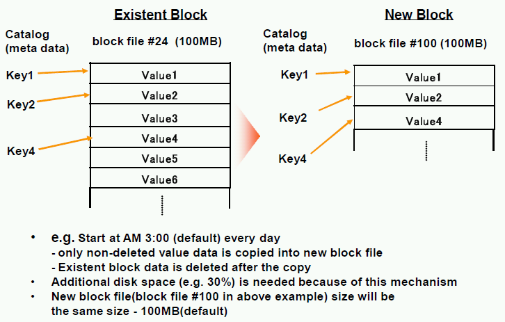
The value of the |
Additional disk space is required to log all updates that
are made after the scavenger has run. This includes space in the
common log as well as in each logical brick private logs (subject to
the general limit of the |
The current implementation of Hibari requires that
plenty of disk space always be available for write-ahead logs and
for scavenger operations. We strongly recommend that the
|
A table can be added at any time, using either of two methods:
- Use the Admin Server’s HTTP service: follow the "Add a table" hyperlink at the bottom of the top-level page.
-
Use the
brick_adminCLI interface at the Erlang shell. See Hibari Contributor’s Guide, "Add a New Table" section.
The current Hibari implementation does not support removing a table. |
In theory, most of the work of removing a table is already done: chains that are abandoned after a migration are shut down * Brick pinger processes are stopped. * Chain monitor processes are stopped. * Bricks are stopped. * Brick data directories are removed.
All that remains is to update the Admin Server’s schema to remove references to the table.
The Hibari Admin Server manages each chain as an independent data replication entity. Though Hibari clients view multiple chains that are associated with a single table, each chain is actually independent of the other chains. It is possible to change the length of one chain without changing any others. For long term operation, such differences do not make sense. But during short periods of cluster reconfiguration, such differences are possible.
A chain’s length is determined by specifying a list of bricks that are
members of that chain. The order of the list specifies the exact
chain order when the chain is in the healthy state. By adding or
removing bricks from a chain definition, the length of the chain can
be changed.
A chain is defined by the Erlang 2-tuple of
{ChainName, ListOfBricks}, where each brick in ListOfBricks is a
2-tuple {BrickName, NodeName}. For example, a chain of length two
called footab_ch1 could be defined as:
{footab_ch1, [{footab1_ch1_b1, 'gdss1@box-a'}, {footab1_ch1_b1, 'gdss1@box-b'}]}The current definition of all chains for table TableName can be
retrieved from the Admin Server using the
brick_admin:get_table_chain_list() function, for example:
%% Get a list of all tables currently defined.
> brick_admin:get_tables().
[tab1]
%% Get list of chains in 'tab1' as they are currently in operation.
> brick_admin:get_table_chain_list(tab1).
{ok,[{tab1_ch1,[{tab1_ch1_b1,'gdss1@machine-1'},
                {tab1_ch1_b2,'gdss1@machine-2'}]},
     {tab1_ch2,[{tab1_ch2_b1,'gdss1@machine-2'},
                {tab1_ch2_b2,'gdss1@machine-1'}]}]}
This above chain list for table tab1 corresponds to the chain and
brick layout below.

To change the definition of a chain, use the
|
When specifying a new chain definition, at least one brick from the current chain must be included. |
The same brick repair technique is used to handle all three of the following cases:
- adding a brick to a chain
- brick failure
- removing a brick from a chain
When a brick B is added to a chain, that brick is treated as if it
was a member of the chain that had crashed long ago and has now been
restarted. The same repair algorithm is used to synchronize data on
brick B that is used to repair bricks that were formerly in service
but since crashed and restarted. See Section 8.5, “Chain Repair” for a
description of the Hibari repair mechanism.
If a brick fails, the Admin Server must remove it from the chain by reordering the chain. The general order of operations are:
- Set new roles for the chain’s bricks, starting from the end of the chain and working backward.
- Broadcast the new chain membership to all Hibari clients.
If a Hibari client attempts to send an operation to a brick during step #2 and before the new chain info from step #2 arrives, that client may send the operation to the wrong brick. Hibari servers will automatically forward the query to the correct brick. Due to network latencies and asynchronous message passing, it is possible that the query be forwarded multiple times before it arrives at the correct brick.
Specific details of how chain replication handles brick failure can be found in van Renesse and Schneider’s paper, see Section 5.3, “Chains” for citation details.
If the head brick fails, then the first middle brick is promoted to the head role. If there is no middle brick (i.e. the length of the chain was two), then the tail brick is promoted to a standalone role (chain length is one).
If the tail brick fails, then the last middle brick is promoted to the tail role. If there is no middle brick (i.e. the length of the chain was two), then the head brick is promoted to a standalone role (chain length is one).
The failure of a middle brick requires the most complex recovery procedure.
Assume that the chain is three bricks:
A→B→C.-
If the chain is longer (more bricks upstream of
Aand/or more bricks downstream ofC), the procedure remains the same.
-
If the chain is longer (more bricks upstream of
-
Brick
Cis configured to have its upstream brick beA. -
Brick
Ais configured to have its downstream brick beC. -
The head of the chain (brick
Aor the head brick upstream ofA) requests a log flush of all unacknowledged writes downstream. This step is required to re-send updates that were processed byAbut have not been received byCbecause of middle brickB's failure. -
Brick
Awaits until it receives a write acknowledgment from the tail of the chain. Once received, all bricks in the chain have synchronously written all items to their write-ahead logs in the correct order.
Removing a brick B permanently from a chain is a simple operation.
Brick B is
handled the same way that any other brick failure is handled: the
chain is simply reconfigured to exclude B. See
Figure 11, “Chain order after a middle brick fails and is repaired (but not yet reordered)” for an example.
When a brick |
There are several cases where it is desirable to rebalance data across chains and bricks in a Hibari cluster:
- Chains are added or removed from the cluster
- Brick hardware is changed, e.g. adding extra disk or RAM capacity
- A change in a table’s consistent hashing algorithm configuration forces data (by definition) to another chain.
The same technique is used in all of these cases: chain migration. This mirrors the same design philosophy that’s used for handling chain changes (see the section called “Chain changes: same algorithm, different tasks.”): use the same algorithm to handle multiple use cases.

In the example above, both the 3-chain and 4-chain configurations used equal weighting factors. When all chains use the same weighting factor (e.g. 100), then the consistent hashing map in the “before” and “after” cases look something like the figure below.

It doesn’t matter that chain #4’s total area within the unit interval is divided into three regions. What matters is that chain #4’s total area is equal to the regions of the other three chains.
The diagram Figure 14, “Migration from three chains to four chains” demonstrates how a migration would work when all chains have an equal weighting factor, e.g. 100. If instead, the new chain had a weighting factor of only 50, then the distribution of keys to each chain would look like this:
Table 2. Migration from three chains to four with unequal chain weighting factors
| Chain Name | Total % of keys before/after migration | Total unit interval size before/after migration |
|---|---|---|
Chain 1 | 33.3% → 28.6% | 100/300 → 100/350 |
Chain 2 | 33.3% → 28.6% | 100/300 → 100/350 |
Chain 3 | 33.3% → 28.6% | 100/300 → 100/350 |
Chain 4 | 0% → 14.3% (4.8% in each of 3 regions) | 0/300 → 50/350 (spread across 3 regions) |
Total | 100% → 100% | 300/300 → 350/350 |
For the original three chains, the total amount of unit interval devoted to those chains is (100+100+100)/350 = 300/350. The 4th chain, because its weighting is only 50, would be assigned 50/350 of the unit interval. Then, an equal amount of unit interval is taken from the original chains and reassigned to chain #4, so (50/350)/3 of the unit interval must be taken from each original chain.
With the lowest level API, it is possible to assign "hot" keys to specific chains, to try to balance a handful of keys that are very frequently accessed from a large number of keys that are very infrequently accessed. The table below gives an example that builds upon Figure 14, “Migration from three chains to four chains”. We assume that our "hot" key is mapped onto the unit interval at position 0.5.
Table 3. Consistent hashing lookup table with three chains of equal weight and a fourth chain with an extremely small weight
| Unit interval start | Unit interval end | Chain name |
|---|---|---|
0.000000 | 0.333333… | Chain 1 |
0.333333… | 0.5 | Chain 2 |
0.5 | 0.500000000000001 | Chain 4 |
0.500000000000001 | 0.666666… | Chain 2 |
0.666666… | 1.0 | Chain 3 |
The table above looks almost exactly like the "Before Migration" half of Figure 14, “Migration from three chains to four chains”. However, there’s a very tiny "hole" that is punched in chain #2’s space that maps key hashes in the range of 0.5 to 0.500000000000001 to chain #4.
It is not strictly necessary to formally configure a list of all Hibari client nodes that may use a Hibari cluster. However, practically speaking, it is useful to do so.
To bootstrap itself to be able to use Hibari servers, a Hibari client must be able to:
- Communicate with other Erlang nodes in the cluster.
- Receive "global hash" information from the cluster’s Admin Server.
To solve both problems, the Admin Server maintains a list of Hibari
client nodes. (Hibari server nodes do not need this mechanism.) For
each client node, a monitor process on the Admin Server polls the node
to see if the gdss or gdss_client application is running. If the
client node is running, then problem #1 (connecting to other nodes in
the cluster) is automatically solved by using net_adm:ping/1.
Problem #2 is solved by the client monitor calling
brick_admin:spam_gh_to_all_nodes/0.
The Admin Server’s client monitor runs approximately once per second, so there may be a delay of up to a couple of seconds before a newly-started Hibari client node is connected to the rest of the cluster and has all of the table info required to start work.
When a client node goes down, an OTP alarm is raised until the client is up and running again.
Two methods can be used to view and change the client node monitor list:
- Use the Admin Server’s HTTP service: follow the "Add/Delete a client node monitor" hyperlink at the bottom of the top-level page.
Use the Erlang CLI to use these functions:
-
brick_admin:add_client_monitor/1 -
brick_admin:delete_client_monitor/1 -
brick_admin:get_client_monitor_list/0
-
For multi-node Hibari deployments, Hibari includes a network monitoring feature that watches for partitions within the cluster, and attempts to minimize the database consequences of such partitions. This Erlang/OTP application is called the Partition Detector.
You can configure the network monitoring feature in the central.conf
file. See Section 7.2, “Parameters in the central.conf File” for details.
Use of this feature is mandatory for a multi-node Hibari deployment to prevent data corruption in the event of a network partition. If you don’t care about data loss, then as an ancient Roman might say, “Caveat emptor.” Or in English, “Let the buyer beware.” |
For the network monitoring feature to work properly, you must first set up two separate networks, Network A and Network B, that connect to each of your Hibari physical bricks. The networks must be set up as follows:
- Network A and Network B must be physically separate networks, with different IP and broadcast addresses. See the diagram below for a two node cluster.
- Network A must be the network used for all Hibari data communications.
- Network A should have as few physical failure points as possible. For example, a single switch or load balancer is preferable to two switches cabled together.
- The separate Network B will be used to compare node heartbeat patterns.
For the network partition monitor to work properly, your network partition monitor configuration settings must match as closely as possible. Each Hibari physical brick must have unique IP addresses on its two network interfaces (as required by all IP networks), but all configurations must use the same IP subnets for the A and B networks, and all configurations must use the same network A tiebreaker. |

Through the partition monitoring application, Hibari nodes send
heartbeat messages to one another at the configurable
heartbeat_beacon_interval, and each node keeps track of heartbeat
history from each of the other nodes in the cluster. The heartbeats
are transmitted through both Network A and Network B. If node
gdss1@machine1 detects that the incoming heartbeats from
gdss1@machine2 are absent both on Network A and on Network B, then
gdss1@machine2 might have a problem. If the incoming heartbeats from
gdss1@machine2 fail on Network A but not on Network B, a partition on
Network A might be the cause. If heartbeats fail on Network B but not
Network A, then Network B might have a partition problem, but this is
less serious because Hibari data communication does not take place on
Network B.
Configurable timers on each Hibari node determine the interval at
which the absence of incoming heartbeats from another node is
considered a problem. If on node gdss1@machine1 no heartbeat has been
received from gdss1@machine2 for the duration of the configurable
heartbeat_warning_interval, then a warning message is
written to the application log of node gdss1@machine1. This warning
message can be triggered by missing heartbeats either on Network A or
on Network B; the warning message will indicate which node has not
been heard from, and over which network.
If on node gdss1@machine1 no heartbeat has been received from
gdss1@machine2 via Network A for the duration of the configurable
heartbeat_failure_interval, and if during that period heartbeats
from gdss1@machine2 continue to be received via Network B, then a
network partition is presumed to have occurred in Network A. In this
scenario, node gdss1@machine1 will attempt to ping the configurable
network_a_tiebreaker address. If gdss1@machine1 successfully pings
the tiebreaker address, then gdss1@machine1 considers itself to be
on the "correct" side of the Network A partition, and it continues
running. If by contrast gdss1@machine1 cannot successfully ping the
tiebreaker address, then gdss1@machine1 considers itself to be on
the "wrong" side of the Network A partition and shuts itself
down. Meanwhile, comparable calculations and decisions are being made
by node gdss1@machine2.
In a scenario where the network monitoring application determines that a partition has occurred on Network B — that is, heartbeats are received through Network A but not through Network B — then warnings are written to the Hibari nodes' application logs but no node is shut down.
At the time of writing, Hibari’s largest cluster deployment is:
- Well over 50 physical bricks
- Well over 4TB of disk space per physical brick
- Single data center, operated by a telecom carrier and integrated with third-party monitoring and control software
If a backup were made of all data in the cluster, the biggest question is, "Where would you store the backup?" Given the cluster’s purpose (real-time email/messaging services), the quality of the data center’s physical and software infrastructures, the length of the Hibari chains used for physical data redundancy, the business factors influencing the choice not to deploy a "hot backup" data center, and other factors, Cloudian has not developed the backup and recovery software for Hibari. Cloudian’s smaller Hibari deployments also resemble the largest deployment.
However, we expect that backup and recovery software will be high priorities for open source Hibari users. Together with the open source users and developers, we expect this software to be developed relatively quickly.
It is certainly possible to deploy a single Hibari cluster across two (or more) data centers. At the moment, however, there is only one way of doing it: each chain of data replication must have a brick located in each data center.
As a consequence of brick placement, it is mandatory that Hibari clients pay the full round-trip latency penalty for each update. See Figure 3, “Message flow in a chain for a key update” for a diagram; the "head" and "tail" bricks would be in separate data centers, using WAN network connectivity between them.
For some applications, strong consistency is a higher priority than low latency (both for writes and possibly for reads, if the client is not co-located in the same data center as the chain’s tail brick). In those cases, such cross-data-center brick placement can make sense.
However, Hibari’s Admin Server cannot handle all failure scenarios, especially when WAN connectivity is broken between data centers; more programming work is required for the Admin Server to automate the handling of all processes. Furthermore, Hibari’s basic design cannot tolerate network partitions well, see Section 1.6, “The CAP Theorem and Hibari” and Section 6.4, “Admin Server and Network Partition”. If the Admin Server were capable of handling WAN network partitions, it’s almost certain that all Hibari nodes in one of the partitioned data centers would be inactive.
Conceptually, it’s possible to run multiple Hibari clusters, one per data center. However, Hibari does not have the software required for WAN-scale replication.
In theory, such software isn’t too difficult to develop. The tail brick of each chain can maintain a log of recent updates to the chain. Those updates can be transmitted asynchronously across a WAN to another Hibari cluster in a remote data center. Such a scheme is depicted in the figure below.

This kind of replication makes the most sense if "Data Center #1"
were in an active role and Data Center #2" were in a hot-standby
role. In that case, there would never be a "Data Center #2 Client",
so there would be no problem of strong consistency violations by
clients accessing both Hibari clusters simultaneously. The only
consistency problem would be one of durability: the replay of async
update logs every N seconds would mean that up to N seconds of
updates within "Data Center #1" could be lost.
However, if clients access both Hibari clusters simultaneously, then Hibari’s strong consistency guarantee would be violated. Some applications can tolerate weakened consistency. Other applications, however, cannot. For the those apps that must have strong consistency, Hibari will require additional design and code.
A keen-eyed reader will notice that Figure 16, “A future scenario of asynchronous, cross-data-center Hibari replication” is not fully symmetric. If clients in "Data Center #2" make updates to the chain, then the same async update log maintenance and replay to "Data Center #1" would also be necessary. |
The Hibari application log records application-related alerts, warnings, and informational messages, as well as trace messages for debugging. By default the application log is written to this file:
<GDSS_HOME>/var/log/gdss-app.log
Each log entry in the Hibari application log is composed of these fields in this order, with vertical bar delimitation:
<PID>|<<ERLANGPID>>|<DATETIME>|<MODULE>|<LEVEL>|<MESSAGECODE>|<MESSAGE>
This Hibari application log entry format is not configurable. Each of these application log entry fields is described in the table that follows. The “Position” column indicates the position of the field within a log entry.
| Position | Field | Description |
|---|---|---|
1 |
| System-assigned process identifier (PID) of the process that generated the log message. |
2 |
| Erlang process identifier. |
3 |
| Timestamp in format |
4 |
| The internal component with which the message is associated. This field is set to a minimum length of 13 characters. If the module name is shorter than 13 characters, spaces will be appended to the module name so that the field reaches the 13 character minimum. |
5 |
| The severity level of the message. The level will be one of the following: |
6 |
| Integer code assigned to all messages of severity level |
7 |
| The message itself, describing the event that has occurred. |
Items written to the Hibari application log come from multiple sources:
- The Hibari OTP application
- Other OTP applications bundled with Hibari
-
Other OTP applications within the Erlang runtime system,
e.g.
kernelandsasl.
The <MESSAGE> field is free-form text. Application code can freely
add newline characters and various white-space padding wherever it
wishes. However, the file format dictates that a newline character
(ASCII 10) appear only at the end of the entire app log message.
The Hibari error logger must therefore reformat the text of the
<MESSAGE> field to remove newlines and to remove whitespace
padding. The result is not nearly as readable as the formatting
presented to the Erlang shell. For example, within the shell, a
message can look like this:
=PROGRESS REPORT==== 12-Apr-2010::17:49:22 ===
          supervisor: {local,sasl_safe_sup}
             started: [{pid,<0.43.0>},
                       {name,alarm_handler},
                       {mfa,{alarm_handler,start_link,[]}},
                       {restart_type,permanent},
                       {shutdown,2000},
                       {child_type,worker}]
Within the Hibari application log, however, the same message is reformatted as line #2 below. The reformatted version is much more difficult for a human to read than the version above, but the purpose of the app log file is to be machine-parsable, not human-parsable.
8955|<0.54.0>|20100412174922|gmt_app      |INFO|2190301|start: normal []
8955|<0.55.0>|20100412174922|SASL         |INFO|2199999|progress: [{supervisor,{local,gmt_sup}},{started,[{pid,<0.56.0>},{name,gmt_config_svr},{mfa,{gmt_config_svr,start_link,["../priv/central.conf"]}},{restart_type,permanent},{shutdown,2000},{child_type,worker}]}]
8955|<0.55.0>|20100412174922|SASL         |INFO|2199999|progress: [{supervisor,{local,gmt_sup}},{started,[{pid,<0.57.0>},{name,gmt_tlog_svr},{mfa,{gmt_tlog_svr,start_link,[]}},{restart_type,permanent},{shutdown,2000},{child_type,worker}]}]
8955|<0.36.0>|20100412174922|SASL         |INFO|2199999|progress: [{supervisor,{local,kernel_safe_sup}},{started,[{pid,<0.59.0>},{name,timer_server},{mfa,{timer,start_link,[]}},{restart_type,permanent},{shutdown,1000},{child_type,worker}]}]
[...skipping ahead...]
8955|<0.7.0>|20100412174923|SASL         |INFO|2199999|progress: [{application,gdss},{started_at,gdss_dev2@bb3}]
8955|<0.98.0>|20100412174923|DEFAULT      |INFO|2199999|brick_sb: Admin Server not registered yet, retrying
8955|<0.65.0>|20100412174923|SASL         |INFO|2199999|progress: [{supervisor,{local,brick_admin_sup}},{started,[{pid,<0.98.0>},{name,brick_sb},{mfa,{brick_sb,start_link,[]}},{restart_type,permanent},{shutdown,2000},{child_type,worker}]}]
8955|<0.105.0>|20100412174924|DEFAULT      |INFO|2199999|top of init: bootstrap_copy1, [{implementation_module,brick_ets},{default_data_dir,"."}]
8955|<0.105.0>|20100412174924|DEFAULT      |INFO|2199999|do_init_second_half: bootstrap_copy1
8955|<0.79.0>|20100412174924|SASL         |INFO|2199999|progress: [{supervisor,{local,brick_brick_sup}},{started,[{pid,<0.105.0>},{name,bootstrap_copy1},{mfa,{brick_server,start_link,[bootstrap_copy1,[{default_data_dir,"."}]]}},{restart_type,temporary},{shutdown,2000},{child_type,worker}]}]
8955|<0.105.0>|20100412174924|DEFAULT |INFO|2199999|do_init_second_half: bootstrap_copy1 finishedAs noted in Section 1.3, “Hibari’s Origins”, at the time of writing, Hibari has been deployed exclusively in data centers run by telecom carriers. All carriers have very specific requirements for integrating with its existing deployment, network monitoring, alarm management, and other infrastructures. As a result, many of those features have been omitted to date from Hibari. With Hibari’s release into an "open source environment", we expect that these gaps will be closed.
Hibari’s carrier-centric heritage has also influenced the types of hardware, networking gear, operating system, support software, and internal Hibari configuration that have been used successfully to date. Some of these practices will change as Hibari evolves from its original use patterns. Until then, this section discusses some of the things that a systems/network administrator must consider when deploying a Hibari cluster.
Similarly, application developers must be very familiar with these same issues. An unaware developer can create an application that uses too many resources on under-specified hardware, causing problems for developers, support staff, and application users alike. We wish Hibari to grow and flourish in its non-relational DB niche.
Each Hibari logical brick stores all information about its keys in RAM. Both the logical brick’s private write-ahead log and the common write-ahead log are not "disk-based data structures" in the typical sense, such as on-disk hash tables or B-trees. Therefore, Hibari bricks require a lot of RAM to function.
For more details, see:
- Section 2.8, “High performance”
- Section 2.14, “Per-table configurable performance options” … if a table stores its value blobs in RAM, it will consume more RAM than if those value blobs are stored on disk.
- Section 4.2, “The Hibari Data Model”
- Section 8.4, “Brick Initialization”
By default, Hibari will write and flush each update to disk before sending a reply downstream or back to the client. Hibari will perform better on systems that have higher disk I/O capacity.
- Non-volatile/battery-backed cache on the disk controller(s) is helpful, when combined with a write-back cache policy. The more cache, the better. If the read/write ratio of the cache can be changed, a default policy of 10/90 or 0/100 (i.e. skewed to writes) is typically more helpful than a default 50/50 split.
- On-disk (volatile) cache on individual disks is not helpful.
- Faster spinning disks are more helpful than slower spinning disks.
- If using RAID, a large stripe width of e.g. 512KBytes or 1024KBytes is usually more helpful than the (usually) smaller default stripe width on most controllers.
- If using RAID, a hardware RAID implementation may be very slightly helpful.
- RAID redundancy (e.g. RAID 1, 10, 5, 6) is not required by Hibari, but it can help reduce the odds of failure of an individual physical brick. If physical bricks do not use data redundant RAID (e.g. RAID 0, concatenation), it’s a good idea to consider using longer replication chains to compensate.
For more details, see:
Hibari has some support for high I/O rate devices such as solid state disks, flash memory disks, flash memory storage cards, et al. There is nothing in Hibari’s implementation that would preclude using high-speed disk devices as the only storage for Hibari write-ahead logs.
Hibari has a feature that can segregate high write I/O with fsync(2)
operations onto a separate high-speed device, and use cheaper &
lower-speed Winchester disk devices for bulk storage. This feature
has not yet been well-tested and optimized.
For more details, see:
More disks of smaller capacity are almost always more helpful than a few disks of larger capacity. RAID 0 (no data redundancy) or RAID 10 ("mirror" data redundancy) is useful for combining the I/O capacity of multiple disks into a single logical volume. Other RAID levels, such as 5 or 6, can be used, though at the expense of higher write I/O overhead.
For more details, see:
Hibari storage bricks do not, as a general rule, require large amounts of CPU capacity. The largest single source of CPU consumption is in MD5 checksum calculation. If the data objects most commonly written & read by your application are small, then multi-socket, multi-core CPUs are not required.
Each Hibari logical brick is implemented within the Erlang virtual
machine as a single gen_server process. Therefore, each logical
brick can (generally speaking) only fully utilize one CPU core. If
your Hibari cluster appears to have CPU-utilization imbalance, then
the recommended strategy is to change the chain placement policy of
the chains. For example, there are two methods for arranging a chain
of length three across three physical bricks:
The first example shows one chain striped across three physical bricks. If the read/write ratio for the chain is extremely high (i.e. most operations are reads), then most of the CPU activity (and perhaps disk I/O, if blobs are stored on disk) will be directed to the "Chain 1 tail" brick and cause a CPU utilization imbalance.
One chain striped across three physical bricks.
| Physical Brick X | Physical Brick Y | Physical Brick Z |
----------------------------------------------------------
   Chain 1 head   ->  Chain 1 middle ->  Chain 1 tail
The second example shows the same three physical bricks but with three chains striped across them. In this example, each physical brick is responsible for three different roles: head, middle, and tail. Regardless of the read/write operation ratio, all bricks will utilize roughly the same amount of CPU.
Three chains striped across three physical bricks.
| Physical Brick T | Physical Brick U | Physical Brick V |
----------------------------------------------------------
   Chain 1 head   ->  Chain 1 middle ->  Chain 1 tail   ||
   Chain 2 tail   ||  Chain 2 head   ->  Chain 2 middle ->
   Chain 3 middle ->  Chain 3 tail   ||  Chain 3 head   ->
In multi-CPU and multi-core systems, a side-effect of using more chains (and therefore more bricks) is that the Erlang virtual machine can schedule more logical brick computation across a larger number of cores and CPUs.
Hibari works quite well using commodity "Gigabit Ethernet" interfaces. Lower latency (and higher cost) networking gear, such as Infiniband, is not required.
For production use, it is strongly recommended that all Hibari servers be configured with two physical network interfaces, cabling, switches, etc. For more details, see:
The native Erlang client, via the gdss or gdss_client OTP
applications, do not require any load balancing. The Erlang client
already is a participant in the consistent hashing algorithm (see
the section called “Partitioning by consistent hashing”). The Admin Server distributes
updates to a table’s consistent hash map each time cluster membership
or chain/brick status changes.
All other client access protocols are "dumb", by comparison. Take for example the Amazon S3 protocol service. There is no easy way for a Hibari cluster to convey to a generic HTTP client how to calculate which brick to send a query to. The HTTP redirect mechanism could be used for this purpose, but other protocols don’t have an equivalent feature. Also, the latency overhead of sending a redirect is far higher than Hibari’s solution to this problem.
Hibari’s solution is simple: the Hibari server-side "dumb" protocol handler uses the same native Erlang client that any other Hibari client app written in Erlang users. That client is capable of making direct routing decisions. Therefore, the "dumb" protocol handler within a Hibari node acts as a translating proxy: it uses the "dumb" client access protocol on one side and uses the native Erlang client API on the other.

The deployed "state of the art" for such dumb protocols is to use a TCP load balancer (aka a "layer 4" load balancer) to spread dumb client workload across multiple Hibari dumb protocol servers.
Hibari servers operate on top of the Erlang virtual machine. In principle, any operating system that is supported by the Erlang virtual machine can support Hibari.
In practice, Hibari is supported on the following operating systems:
- Linux (used in production and QA environments within Cloudian, Inc.)
- Mac OS X
- FreeBSD (though not currently in a jail environment, due to some TCP services getting EPROTONOSUPPORT errors)
To take advantage of RAM larger than 3.0, 3.5, or 4.0 gigabytes (depending on the OS kernel), we recommended that you use a 64-bit version of your OS’s kernel, 64-bit versions of the user runtime, and a 64-bit version of the Erlang/OTP runtime.
Some operating systems have support for OS-based "readahead": pre-fetching blocks of a file with the expectation that those blocks will soon be requested by the application. Properly configured, readahead can substantially raise throughput and reduce latency on many read-heavy I/O workloads.
The read I/O workloads for Hibari fall into two major categories:
- Extremely predictable sequential read-only I/O during brick initialization (see Section 8.4, “Brick Initialization”).
- Extremely unpredictable random read I/O for fetching value blobs from disk.
The first I/O pattern can usually benefit a great deal from an aggressive readahead policy. However, an aggressive readahead policy can have the opposite effect on the second I/O pattern. Readahead policies under Linux, for example, are defined on a per-block device basis and does not change in response to application runtime behavior.
If your OS supports readahead policy configuration, we recommend using a small read and then measuring its effect with a real or simulated workload with the real Hibari server.
A typical "server" type installation of a Linux or FreeBSD OS is sufficient for Hibari. The following is an incomplete list of other software packages that are necessary for Hibari’s installation and/or runtime.
- NTP
- Erlang/OTP version R13B04
- Either "lynx" or "elinks", a text-based Web browser
It is strongly recommended that all Hibari server and client nodes have the NTP daemon (Network Time Protocol) installed, properly configured, and running.
-
The
brick_simpleclient API uses the OS clock for automatic generation of timestamps for each key update. The application problems caused by badly out-of-sync OS clocks can be easily avoided by NTP. If a client’s clock is skewed by more than the
brick_do_op_too_old_timeoutconfiguration attribute incentral.conf(units = milliseconds), then the brick will silently discard the client’s operation. The only symptoms of this are:-
Client-side timeouts when using the
brick_simple,brick_server, orbrick_squorumAPIs. -
Increasing
n_too_oldstatistic counter on the brick.
-
Client-side timeouts when using the
There are several reasons why disk I/O rates can temporarily increase within a Hibari physical brick:
- Logical brick checkpoints for increased write I/O ops, see Section 8.6, “Brick Checkpoint Operations”
- The common log "scavenger" for increased read and write I/O ops, see Section 8.7, “The Scavenger”
Chain replication repair, see Section 8.5, “Chain Repair”
- As the upstream/"repairer" brick, the extra read I/O ops, if the brick stores value blobs on disk
- As the downstream/"repairee" brick, extra write I/O ops
The Hibari central.conf file contains parameters that can limit the
amount of disk bandwidth used by most of these operations.
See also:
The Admin Server’s status page contains current status information regarding all tables, chains, and bricks in the cluster. By default, this service listens to TCP port 23080 and is reachable via HTTP at http://any-hibari-node-name:23080/. HTTP redirect will steer your browser to the Admin Server node.
- Hypertext links for each table, chain, and brick can show more detailed info on each entity.
- The "Dump History" link at the bottom of the Admin Server’s HTTP status page can show operations history across multiple bricks, chains, and/or tables by using the regular expression feature.
Each logical brick maintains counters of each type of Hibari client op primitive. At present, these stats are only exposed via the HTTP status server or by the native Erlang interface, but it’s possible to expose these stats via SNMP and other protocols in a straightforward manner.
-
Stats include: number of
add,replace,set,get,get_many,delete, and micro-transactions.
-
Stats include: number of
For example screen shots of the Admin Server status pages (a work in progress), see ./misc-screenshots/admin-server-status/index.html.
See also:
- Add a new table
- Delete a table
Change to a single chain:
- Add one or more bricks (increase replication factor)
- Remove one or more bricks (decrease replication factor)
Change to a single table.
- Add a new chain
- Remove a chain
- Change the chain weighting factor
- Change consistent hashing parameters
Hash prefixes allow Hibari servers to guarantee the application developer that certain keys will always be stored on the same chain and therefore always on the same set of bricks. With this guarantee, an application aware of hash prefixes can use micro-transactions successfully.
For example, assume the application requires a collection of persistent stacks that are stored in Hibari.
- Each stack is identified by a string/binary. (The two types are identical for the sake of discussion.)
- Each item stored on the stack is a string.
- Support stack options push & pop.
- Support quick stack stats, e.g. # of elements on the stack and # of bytes stored on the stack.
- Stacks may contain hundreds of thousands of items.
- The total size of a stack will not exceed the total storage capacity of any single brick in the cluster.
Understanding the last assumption is vital. Because all
keys with the same hash prefix |
The application developer then makes the following decisions:
-
The application will use a table devoted to storing stacks, called
'stack'. -
We know that the application requires strong durability (which is
the Hibari default) and that the sum total of all stack items will
exceed a single brick’s RAM capacity. Therefore, the
'stack'table must store its value blobs on disk. Read access to the table will be slower than if value blobs were stored in RAM, but the limited RAM capacity of bricks does not give us a choice. We have two machines,
boxAandboxB, available for hosting the table’s logical bricks. We want to be able to survive at least one physical brick failure, therefore all chains have a minimum length of 2.- We will use two chains, so that each physical machine (when up and running smoothly) will have 2 logical bricks for the table, one in the chain head role and one in the chain tail role.
- The naming scheme used for each chain name and brick name can be arbitrary, as long as all names are unique. However, for ease-of-management purposes, the use of a systematic naming scheme is strongly encouraged. The scheme used here numbers each chain (starting at 1) and numbers each brick (also starting at 1) with both the chain and brick number.
We use the following key naming convention:
-
A stack’s metadata (item count, byte count) uses
<<"/StackName/md">>. -
A item uses
<<"/StackName/N">>where N is the item number.
-
A stack’s metadata (item count, byte count) uses
We create the table using the following:
Opts = [{hash_init, fun brick_admin:chash_init/3}, {prefix_method, var_prefix},
        {num_separators, 2}, {prefix_separator, $/},
        {new_chainweights, [{stack_ch1, 100}, {stack_ch2, 100}]},
        {bigdata_dir, "."}, {do_logging, true}, {do_sync, true}].

ChainList = [{stack_ch1, [{stack_ch1_b1, hibari1@boxA},
                          {stack_ch1_b2, hibari1@boxB}]},
             {stack_ch1, [{stack_ch2_b1, hibari1@boxB},
                          {stack_ch2_b2, hibari1@boxA}]}].

brick_admin:add_table(stack, ChainList, Opts).
See the section called “Examples code for using the stack” for sample usage code.
add_table(Name, ChainList)
  equivalent to add_table(brick_admin, Name, ChainList)

add_table(Name, ChainList, BrickOptions)
  when is_atom(Name), is_list(ChainList)
  equivalent to add_table(brick_admin, Name, ChainList, BrickOptions)

add_table(ServerRef, Name, BrickOptions)
  when is_atom(Name), is_list(BrickOptions)
  equivalent to add_table(ServerRef, Name, ChainList, [])

add_table(ServerRef::gen_server_serverref(), Name::table(),
          ChainList::chain_list(), BrickOptions::brick_options())
-> ok |
   {error, term()} |
   {error, term(), term()}

gen_server_serverref() = "ServerRef" type from STDLIB gen_server, gen_fsm, etc.
proplists_property()   = "Property" type from STDLIB proplists

bigdata_option()    = {'bigdata_dir', string()}
brick()             = {logical_brick(), node()}
brick_option()      = chash_prop() |
                      custom_prop() |
                      fixed_prefix_prop() |
                      {'hash_init', fun/3} |
                      var_prefix_prop()
brick_options()     = [brick_option]
chain_list()        = {chain_name(), [brick()]}
chain_name()        = atom()
chash_prop()        = {'new_chainweights', chain_weights()} |
                      {'num_separators', integer()} |
                      {'old_float_map', float_map()} |
                      {'prefix_is_integer_hack', boolean()} |
                      {'prefix_length', integer()} |
                      {'prefix_method', 'all' | 'var_prefix' | 'fixed_prefix'} |
                      {'prefix_separator', integer()}
chain_weights()     = [{chain_name, integer()}]
custom_prop()       = proplists_property()
fixed_prefix_prop() = {'prefix_is_integer_hack', boolean()} |
                      {'prefix_length', integer()}
logging_option()    = {'do_logging', boolean()}
logical_brick()     = atom()
node()              = atom()
sync_option()       = {'do_sync', boolean()}
table()             = atom()
var_prefix_prop()   = {'num_separators', integer()} |
{'prefix_separator', integer()}-
{'bigdata_dir', string()} To store value blobs on disk (i.e. "big data" is true), specify this value with any string (the string’s actual value is not used).
![[Important]](images/icons/important.png)
To store value blobs in RAM, this option must be omitted.
-
{'do_logging', boolean()} - Specify whether all bricks in the table will log updates to disk. If not specified, the default is true.
-
{'do_sync', boolean()} - Specify whether all bricks in the table will synchronously flush all updates to disk before responding to the client. If not specified, the default is true.
-
{'hash_init', fun/3} -
Specify the hash initialization function. Of the four hash methods
bundled with Hibari, we recommend using
brick_hash:chash_init/3only. -
{'new_chainweights, chain_weights()} -
(For
brick_admin:chash_init/3) Specify the chainweights for this new table. For creating a new table, this option is not used. However, this option is used when changing a table to add/remove chains or to change other table-related parameters. -
{'num_separators', integer()} (For
brick_admin:chash_init/3andbrick_admin:var_prefix_init/3) For variable prefix hashes, this option specifies how many instances of the variable prefix separator character (see'prefix_separator'below) are included in the hashing prefix. The default is 2.For example, if
{'prefix_separator', $/}, then-
With
{'num_separators', 2}and key<<"/foo/bar/baz/hello">>, the hashing prefix is<<"/foo/">>. -
With
{'num_separators', 3}and key<<"/foo/bar/baz/hello">>, the hashing prefix is<<"/foo/bar/">>.
-
With
-
{'old_float_map', float_map()} - Specify the old version of the "float map". For creating a new table, this option is not used. However, this option is used when changing a table to add/remove chains or to change other table-related parameters: it is used to create a new mapping of {table, key} → chain that relocates only a minimum number of keys a new chain.
-
{'prefix_method', 'all' | 'var_prefix' | 'fixed_prefix'} (For
brick_admin:chash_init/3) Specify which prefix method will be used for consistent hashing:-
'all': Use the entire key -
'var_prefix': Use a variable-length prefix of the key -
fixed_prefix': Use a fixed-length prefix of the key
-
-
{'prefix_is_integer_hack', boolean()} -
(For
brick_admin:fixed_prefix_init/3) If true, the prefix should be interpreted as an ASCII representation of a base 10 integer for use as the hash calculation. -
{'prefix_length', integer()} -
(For
brick_admin:fixed_prefix_init/3) For a fixed-prefix hashes, this option specifies the prefix length. -
{'prefix_separator', integer()} -
(For
brick_admin:chash_init/3andbrick_admin:var_prefix_init/3) For variable prefix hashes, this option specifies the single byte ASCII value of the byte that separates the key’s prefix from the rest of the key. The default is $/, ASCII 47.
Create a new stack.
Val = #stack_md{count = 0, bytes = 0}.
brick_simple:add(stack, "/new-stack/md", term_to_binary(Val)).
Push an item onto a stack.
{ok, OldTS, OldVal} = brick_simple:get(stack, "/new-stack/md").
#stack_md{count = Count, bytes = Bytes} = binary_to_term(OldVal).
NewMD = #stack_md{count = Count + 1, bytes = Bytes + size(NewItem)}.
ItemKey = "/new-stack/" ++ integer_to_list(Count).
[ok, ok] = brick_simple:do(stack,
                           [brick_server:make_txn(),
                            brick_server:make_replace("/new-stack/md",
                                                      term_to_binary(NewMD),
                                                      0, [{testset, OldTS}]),
                            brick_server:make_add(ItemKey, NewItem)]).
Pop an item off a stack.
{ok, OldTS, OldVal} = brick_simple:get(stack, "/new-stack/md").
#stack_md{count = Count, bytes = Bytes} = binary_to_term(OldVal).
ItemKey = "/new-stack/" ++ integer_to_list(Count - 1).
{ok, _, Item} = brick_simple:get(stack, ItemKey).
NumBytes = proplists:get_value(val_len, Ps).
NewMD = #stack_md{count = Count - 1, bytes = Bytes - size(Item)}.
[ok, ok] = brick_simple:do(stack,
                           [brick_server:make_txn(),
                            brick_server:make_replace("/new-stack/md",
                                                      term_to_binary(NewMD),
                                                      0, [{testset, OldTS}]),
                            brick_server:make_delete(ItemKey)]).
Item.
As yet, Hibari does not have a method to delete a table. The only methods available now are:
-
Delete all files and subdirectories from the
bootstrap_*brick data directories, restart the Admin Server, and recreate all tables. (Also known as, "Start over".) -
Make a backup copy of all
bootstrap_*brick data directories before creating a new table. If you wish to undo, then stop Hibari on all Admin Server-eligible nodes, remove thebootstrap_*brick data directories, restore thebootstrap_*brick data directories from the previous backup, then start all of the Admin Server-eligible nodes.
Adding or removing bricks from a single chain changes the replication factor for the keys stored in that chain: more bricks increases the replication factor, and fewer bricks decreases it.
Data types for brick_admin:change_chain_length().
brick_admin:change_chain_length(ChainName, BrickList)

ChainName       = atom()
BrickList       = [brick()]

brick()         = {logical_brick(), node()}
logical_brick() = atom()
node()          = atom()
See also,
brick_admin:change_chain_length() usage examples
Section 14.9, “Changing Chain Length: Examples”.
Data types for brick_admin:start_migration().
brick_admin:start_migration(TableName, LH)
  equivalent to brick_admin:start_migration(TableName, LH, [])

brick_admin:start_migration(TableName, LH, Options)
-> {ok, cookie()} |
   {'EXIT', term()}

TableName           = atom()
LH                  = hash_r()
Options             = migration_options()

cookie()            = term()
migration_option()  = {'do_not_initiate_serial_ack', boolean()} |
                      {'interval', integer()} |
                      {'max_keys_per_chain', integer()} |
                      {'max_keys_per_iter', integer()} |
                      {'propagation_delay', integer()}
migration_options() = [migration_option()]

brick_admin:chash_init('via_proplist', ChainList, Options)
-> hash_r()

ChainList = chain_list()
Options   = brick_options()
See the section called “Types for brick_admin:add_table()” for definitions of
chain_list() and brick_options() types.
The hash_r() type is an Erlang record, #hash_r as defined in the
brick_hash.hrl header file. It is normally considered an opaque
type that is created by a function such as brick_hash:chash_init/3.
The options list passed in argument #3 to
|
Once a hash_r() term is created and brick_admin:start_migration/2
is called successfully, the data migration will start immediately.
The cookie() type is an opaque term that uniquely identifies the
data migration that was triggered for the TableName table. Another
data migration may not be triggered until the current migration has
finished successfully.
The migration_option() properties are described below:
-
{'do_not_initiate_serial_ack', boolean()} - For internal use only, do not use.
-
{'interval', integer()} - Interval (in milliseconds) to send kick_next_sweep messages. Default = 50.
-
{'max_keys_per_chain', integer()} - Maximum number of keys to send to any particular chain. Not yet implemented.
-
{'max_keys_per_iter', integer()} - Maximum number of keys to examine per sweep iteration. Default = 500 for bricks with value blobs in RAM, 25 for bricks with value blobs on disk.
-
{'propagation_delay', integer()} - Number of milliseconds to delay for each brick’s logging operation. Default = 0.
See also Section 14.10, “Creating and Rebalancing Chains: Examples”.
The functions to change chain weighting are the same for adding/removing chains, see Section 14.4, “Change a Table: Add/Remove Chains” for additional details.
When creating a hash_r() type record, follow these two bits of
advice:
-
The
chain_list()term remains exactly the same as the chain list currently used by the table. Seebrick_admin:get_table_chain_list/1for how to retrieve this list. -
The
new_chainweightsproperty in thebrick_options()list specifies a different set of chain weighting factors than is currently used by the table. The current chain weighting list is in thebrick_optionsproperty returned by thebrick_admin:get_table_info/1function.
See also Section 14.10, “Creating and Rebalancing Chains: Examples”.
The Admin Server’s basic definition of a chain: the chains name, and the list of bricks. In turn, each brick is defined by a 2-tuple of brick name and node name.
Chain definition = {ChainName, [BrickDef1, BrickDef2, ...]}
Brick definition = {BrickName, NodeName}

Example chain definition, chain length=1
    {tab1_ch1, [{tab1_ch1_b1, hibari1@bb3}]}
The function brick_admin:get_table_chain_list/1 will retrieve the
active chain definition list for a table. For example, we retrieve the
chain definition list for the table tab1. The node bb3 is the
hostname of my laptop.
(hibari1@bb3)23> {ok, Tab1ChList} = brick_admin:get_table_chain_list(tab1).
{ok,[{tab1_ch1,[{tab1_ch1_b1,hibari1@bb3}]}]}

(hibari1@bb3)24> Tab1ChList.
[{tab1_ch1,[{tab1_ch1_b1,hibari1@bb3}]}]
The |
To change the chain length, use the
brick_admin:change_chain_length/2 function. The arguments are the
chain name and brick list.
Any bricks in the brick list that aren’t in the chain are automatically started. Any bricks in the current chain that are not in the new list are halted, and their persistent data will be deleted. |
(hibari1@bb3)29> brick_admin:change_chain_length(tab1_ch1,
                 [{tab1_ch1_b1,hibari1@bb3}, {tab1_ch1_b2,hibari1@bb3}]).
ok

(hibari1@bb3)30> {ok, Tab1ChList2} = brick_admin:get_table_chain_list(tab1). {ok,[{tab1_ch1,[{tab1_ch1_b1,hibari1@bb3},
                {tab1_ch1_b2,hibari1@bb3}]}]}
Now the tab1_ch1 chain has length two. We’ll shorten it back down
to length 1.
(hibari1@bb3)31> brick_admin:change_chain_length(tab1_ch1, [{tab1_ch1_b2,hibari1@bb3}]).
ok

(hibari1@bb3)32> {ok, Tab1ChList3} = brick_admin:get_table_chain_list(tab1).
{ok,[{tab1_ch1,[{tab1_ch1_b2,hibari1@bb3}]}]}
A chain’s new brick list must contain at least one brick from the current chain’s definition. If the intersection of old brick list and new brick list is empty, the command will fail. |
(hibari1@bb3)34> brick_admin:change_chain_length(tab1_ch1, [{tab1_ch1_b3,hibari1@bb3}]).
{'EXIT',{error,no_intersection}}The procedure for creating new chains, deleting existing chains, and
reweighing existing chains, and rehashing is done using the the
brick_admin:start_migration() function. The chain definitions are
specified in the same way as changing chain lengths, see
Section 14.9, “Changing Chain Length: Examples” for details.
The data structure required by brick_admin:start_migration/2 is more
complex than the relatively-simple brick list that
brick_admin:change_chain_length/2 requires. This section will
demonstrate the creation of this structure, the “local hash record”,
step-by-step.
First, we create a new chain definition list. (Refer to
Section 14.9, “Changing Chain Length: Examples” if necessary.) For this example, we’ll
assume that we’ll be modifying the tab1 table and that we’ll be
adding two more chains. Each chain will be of length one. We’ll
place each chain on the same node as everything else, hibari1@bb3
(i.e. my laptop).
(hibari1@bb3)48> brick_admin:get_table_chain_list(tab1).
{ok,[{tab1_ch1,[{tab1_ch1_b1,hibari1@bb3}]}]}

(hibari1@bb3)49> NewCL = [{tab1_ch1, [{tab1_ch1_b1, hibari1@bb3}]},
                 {tab1_ch2, [{tab1_ch2_b1, hibari1@bb3}]},
                 {tab1_ch3, [{tab1_ch3_b1, hibari1@bb3}]}].
[{tab1_ch1,[{tab1_ch1_b1,hibari1@bb3}]},
 {tab1_ch2,[{tab1_ch2_b1,hibari1@bb3}]},
 {tab1_ch3,[{tab1_ch3_b1,hibari1@bb3}]}]
Any bricks in the brick list that aren’t in a chain are automatically started. Any bricks in a current chains that are not in the chain definition are halted, and their persistent data will be deleted. |
Next, we retrieve the table’s current hashing configuration. The data
is returned to us in the form of an Erlang property list. (See the
Erlang/OTP documentation for the proplists module, located in the
"Basic Applications" area under "stdlib".) We then pick out several
properties that we’ll need later; we use lists:keyfind/3 instead of
a function in the proplists module because it will preserve the
properties in 2-tuple form, which will save us some typing effort
later.
(hibari1@bb3)51> {ok, TabInfo} = brick_admin:get_table_info(tab1).
{ok,[{name,tab1},
    ...lots of stuff omitted...

(hibari1@bb3)53> Opts = proplists:get_value(brick_options, TabInfo).
[{hash_init,#Fun<brick_hash.chash_init.3>},
 {old_float_map,[]},
 {new_chainweights,[{tab1_ch1,100}]},
 {hash_init,#Fun<brick_hash.chash_init.3>},
 {prefix_method,var_prefix},
 {prefix_separator,47},
 {num_separators,3},
 {bigdata_dir,"cwd"},
 {do_logging,true},
 {do_sync,true},
 {created_date,{2010,4,17}},
 {created_time,{17,21,58}}]

(hibari1@bb3)58> PrefixMethod = lists:keyfind(prefix_method, 1, Opts).
{prefix_method,var_prefix}

(hibari1@bb3)59> NumSep = lists:keyfind(num_separators, 1, Opts).
{num_separators,3}

(hibari1@bb3)60> PrefixSep = lists:keyfind(prefix_separator, 1, Opts).
{prefix_separator,47}

(hibari1@bb3)61> OldCWs = proplists:get_value(new_chainweights, Opts).
[{tab1_ch1,100}]

(hibari1@bb3)62> OldGH = proplists:get_value(ghash, TabInfo).

(hibari1@bb3)63> OldFloatMap = brick_hash:chash_extract_new_float_map(OldGH).
Next, we create a new property list.
(hibari1@bb3)71> NewCWs = OldCWs ++ [{tab1_ch2, 100}, {tab1_ch3, 100}].
[{tab1_ch1,100},{tab1_ch2,100},{tab1_ch3,100}]

(hibari1@bb3)72> NewOpts = [PrefixMethod, NumSep, PrefixSep,
                               {new_chainweights, NewCWs},
                               {old_float_map, OldFloatMap}].
[{prefix_method,var_prefix},
 {num_separators,3},
 {prefix_separator,47},
 {new_chainweights,[{tab1_ch1,100},
                    {tab1_ch2,100},
                    {tab1_ch3,100}]}
 {old_float_map, []}]
Next, we use the chain definition list, NewCL, and the table options
list, NewOpts, to create a “local hash” record. This record will
contain all of the configuration information required to change a
table’s consistent hashing characteristics.
(hibari1@bb3)73> NewLH = brick_hash:chash_init(via_proplist, NewCL, NewOpts).
{hash_r,chash,brick_hash,chash_key_to_chain,
 ...lots of stuff omitted...
We’re just one step away from changing the tab1 table. Before we
change the table, however, we’d like to see how the table change will
affect the data in the table. First, we add 1,000 keys to the tab1
table. Then we use the brick_simple:chash_migration_pre_check/2
function to tell us how many keys will move and to where.
(hibari1@bb3)74> [brick_simple:set(tab1, "foo"++integer_to_list(X), "bar") || X <- lists:seq(1,1000)].
[ok,ok,ok,ok,ok,ok,ok,ok,ok,ok,ok,ok,ok,ok,ok,ok,ok,ok,ok,
 ok,ok,ok,ok,ok,ok,ok,ok,ok,ok|...]

(hibari1@bb3)75> brick_simple:chash_migration_pre_check(tab1, NewLH).
[{keys_before,[{tab1_ch1,1001}]},
 {keys_keep,[{tab1_ch1,348}]},
 {keys_moving,[{tab1_ch2,315},{tab1_ch3,338}]},
 {keys_moving_where,[{tab1_ch1,[{tab1_ch2,315},
                                {tab1_ch3,338}]}]},
 {errors,[]}]
The output above shows us that of the 1,001 keys in the tab1 table,
348 will remain in the tab1_ch1 chain, 315 keys will move to the
tab1_ch2 chain, and 338 keys will move to the tab1_ch3 chain.
That looks like what we want, so let’s reconfigure the table and start
the data migration.
brick_admin:start_migration(tab1, NewLH).
Immediately, we’ll see a bunch of application messages sent to the console as new activities start:
- A migration monitoring process is started.
- New brick processes are started.
- New monitoring processes are started.
- Data migrations are started and finish
- The migration monitoring process exits.
=GMT INFO REPORT==== 20-Apr-2010::00:26:40 ===
Migration number 1 is starting with cookie {1271,741200,988900}

=GMT INFO REPORT==== 20-Apr-2010::00:26:41 ===
progress: [{supervisor,{local,brick_mon_sup}},
           {started,
               [{pid,<0.2937.0>},
                {name,chmon_tab1_ch2},
                ...stuff omitted...

[...lines skipped...]
=GMT INFO REPORT==== 20-Apr-2010::00:26:41 ===
Migration monitor: tab1: chains starting

[...lines skipped...]
=GMT INFO REPORT==== 20-Apr-2010::00:26:41 ===
brick_admin: handle_cast: chain tab1_ch2 in unknown state

[...lines skipped...]
=GMT INFO REPORT==== 20-Apr-2010::00:26:52 ===
Migration monitor: tab1: sweeps starting

[...lines skipped...]
=GMT INFO REPORT==== 20-Apr-2010::00:26:54 ===
Migration number 1 finished

[...lines skipped...]
=GMT INFO REPORT==== 20-Apr-2010::00:26:57 ===
Clearing final migration state for table tab1
For the sake of demonstration, now let’s see what
brick_simple:chash_migration_pre_check() would say if we were to
migrate from three chains to four chains.
(hibari_dev@bb3)24> {ok, TabInfo3} = brick_admin:get_table_info(tab1).

(hibari_dev@bb3)25> Opts3 = proplists:get_value(brick_options, TabInfo3).

(hibari_dev@bb3)26> GH3 = proplists:get_value(ghash, TabInfo3).

(hibari_dev@bb3)28> OldFloatMap = brick_hash:chash_extract_new_float_map(GH3).

(hibari_dev@bb3)31> NewOpts4 = [PrefixMethod, NumSep, PrefixSep,
                    {new_chainweights, NewCWs4}, {old_float_map, OldFloatMap}].

(hibari_dev@bb3)35> NewCL4 = [ {tab1_ch1, [{tab1_ch1_b1, hibari1@bb3}]},
                               {tab1_ch2, [{tab1_ch2_b1, hibari1@bb3}]},
                               {tab1_ch3, [{tab1_ch3_b1, hibari1@bb3}]},
                               {tab1_ch4, [{tab1_ch4_b1, hibari1@bb3}]} ].
(hibari_dev@bb3)36> NewLH4 = brick_hash:chash_init(via_proplist, NewCL4, NewOpts4).

(hibari_dev@bb3)37> brick_simple:chash_migration_pre_check(tab1, NewLH4).
[{keys_before,[{tab1_ch1,349},
               {tab1_ch2,315},
               {tab1_ch3,337}]},
 {keys_keep,[{tab1_ch1,250},{tab1_ch2,232},{tab1_ch3,232}]},
 {keys_moving,[{tab1_ch4,287}]},
 {keys_moving_where,[{tab1_ch1,[{tab1_ch4,99}]},
                     {tab1_ch2,[{tab1_ch4,83}]},
                     {tab1_ch3,[{tab1_ch4,105}]}]},
 {errors,[]}]
The output tells us that chain tab1_ch1 will lose 99 keys,
tab1_ch2 will lose 83 keys, and tab1_ch3 will lose 105 keys. The
final key distribution across the four chains would be 250, 232, 232,
and 287 keys, respectively.